Prediction of Steady-State Flow Fields with Neural Networks

In a CFD simulation, physical problems are described by fluid mechanical equations and solved approximately with numerical methods. This procedure is generally computational intensive and time-consuming. Instead of solving a system of partial differential equations iteratively, the goal is to train a deep learning model that approximates the solution. Convolutional neural networks (CNNs) are suitable for this purpose. The CNN is to learn characteristics describing a flow in order to generate predictions for new cases. In this way, flow fields can be calculated much faster. However, it must be examined how high the quality loss compared to CFD simulations is.

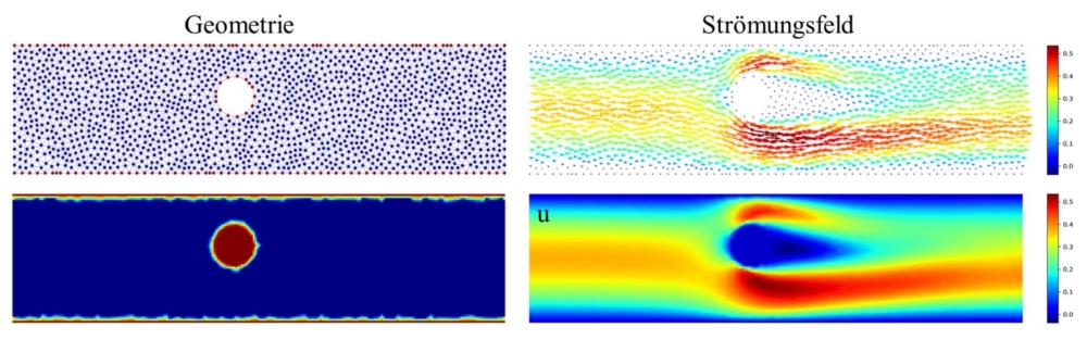
The model used requires an extensive data set for the training process. Significant variation in the data is important in order to learn as many flow phenomena as possible. For this reason, a generic data set is created from CFD simulations. To keep the complexity low, the setup is limited to two-dimensional steady channel flows with different immersed geometries. CNN's cannot handle unstructured CFD grids. Therefore, the data must be interpolated to a Cartesian grid in a preprocessing step. This corresponds to an image, here with 64x256 pixels, where color-channels represent velocities (𝑢,𝑣) and pressure (𝑝). Then, the color-channels are normalized to the range of values [-1,1]. Following the same scheme, the geometry is transferred to an image, where all geometry-nodes represent one and the fluid-elements represent zero. The procedure is illustrated by an exemplary grid in Figure 1.

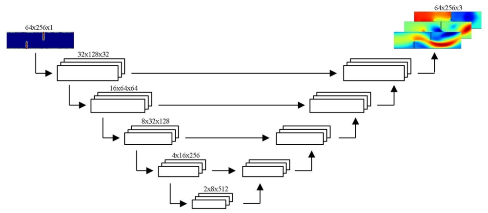
The model for processing geometry information into flow fields is based on the U-Net architecture. This comprises two symmetric paths, shown in Figure 2. In the contraction path, the input data is compressed step by step. In this process, the network learns to extract the spatial information, e.g., position, arrangement, and size of the objects in the data. Then, the data is decompressed again in the expansion path and transformed into a flow field (𝑢,𝑣,𝑝). Cross-connections ensure that contextual information is available at each level of the expansion path.

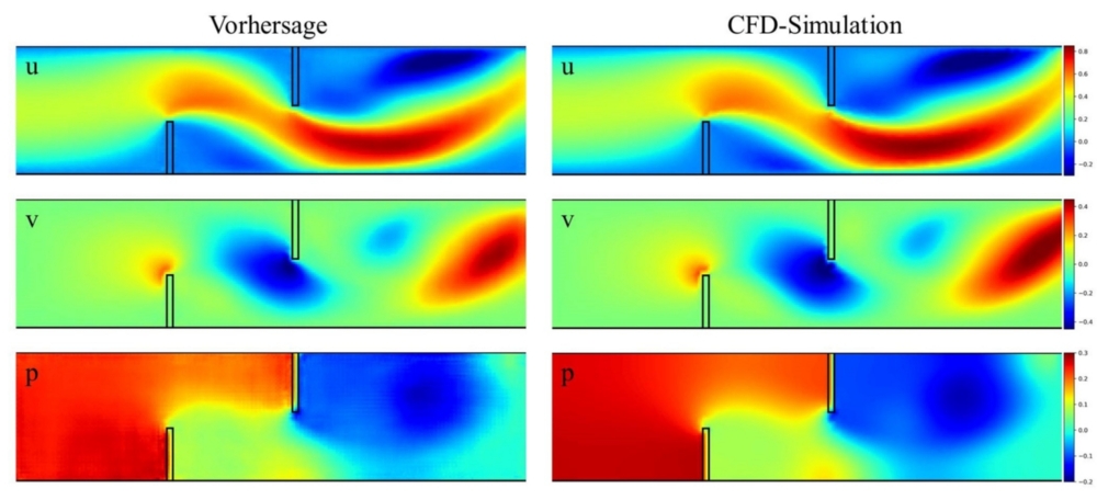
To test the applicability of the trained model to new data (generalization), the U-Net is evaluated with 300 new CFD simulations. For each test sample, a flow field is predicted from the geometry. An example and the corresponding CFD simulation are shown in Figure 3.

For the evaluation of the generalization, the relative error between the predicted values and CFD simulation is calculated. The mean inflow velocity, as well as the given reference pressure, are used as reference variables. The U-Net achieves a relative error of 3.8%, 2%, and 1.1% for (𝑢,𝑣,𝑝), respectively. This shows that a relatively high precision of the individual flow variables can be achieved over the entire channel.